
Thirty minutes, six industrial cases and a single question: how do you go from a measurement to a decision? At Mesures Solutions Expo, the stopwatch forced Luc Desruelle and Amaury Laurent to skim. Here is the long version, with the figures, the curves and the videos they had at hand, and what they chose not to show.
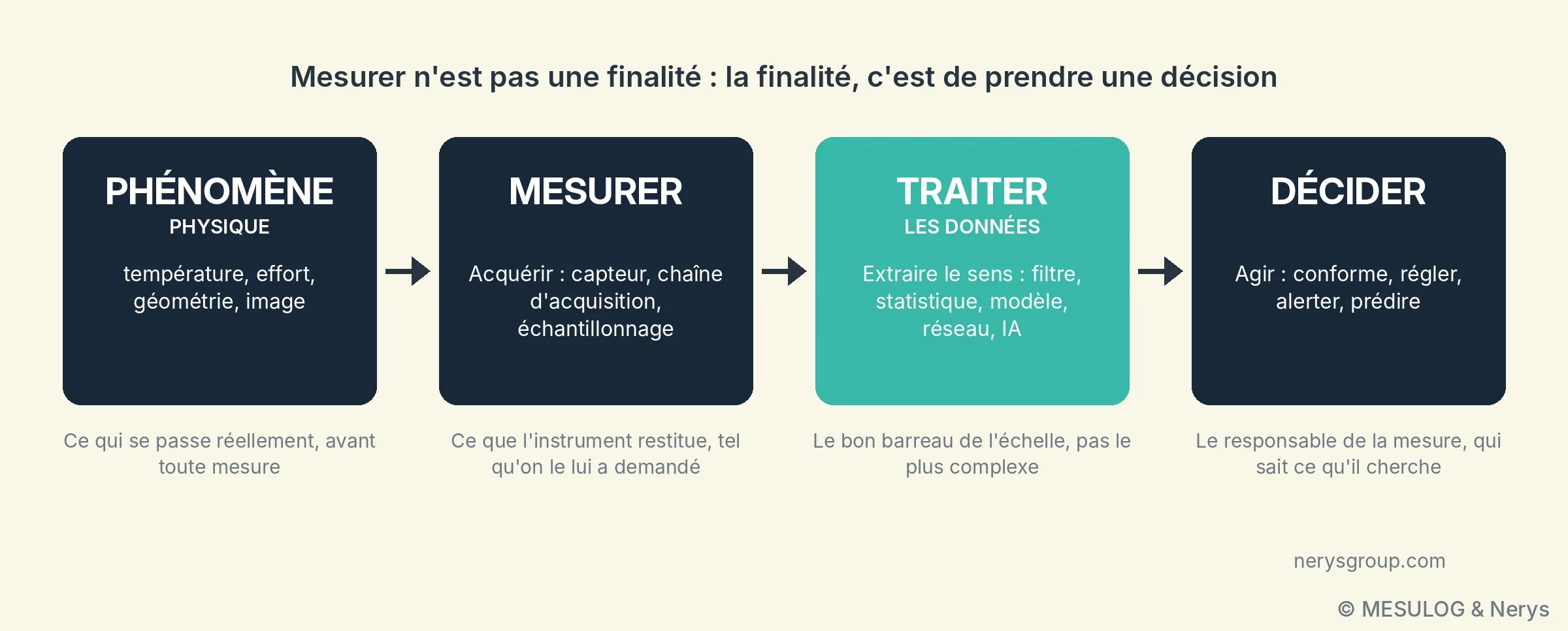
Measuring is not an end in itself. Nobody pays for a test bench to get numbers; they pay to decide: compliant or not, adjust or leave alone, alert or wait, and more and more often, predict. Between the physical quantity and that decision there is processing. That processing is what gives the measurement its value, and it is most often chosen out of habit.
On 15 October, in Lyon, Luc Desruelle, chairman of Mesulog and Nerys, and Amaury Laurent, head of embedded systems and R&D at Nerys, walked through six examples drawn from their projects, from the simplest to the most advanced: a moving average, a process capability, a linear regression on a point cloud, a neural-network camera, an embedded estimator on FPGA designed with Schneider Electric, and a generative AI handed a file of measurements. The common thread fitted in one sentence, repeated after each example: "it worked because we knew what we were looking for". The end of the workshop showed what happens when that is not the case.
1. A temperature: which value to keep?
The simplest case there is, built for the occasion in LabVIEW: the temperature of the Mesures Solutions Expo room, stable around 18 °C. A real measurement is never perfectly stable. It carries noise, and from time to time a frankly aberrant value: interference on the link, a contact that moves, an electromagnetic disturbance when a nearby motor starts.
Mean or median: two hypotheses about the noise
First reflex: smooth with a moving average. In the demonstration, the display goes from a raw measurement of 18.2 °C ± 3.7 °C to a processed value of 18.7 °C ± 0.4 °C: the noise is divided by nine, but the spikes have shifted the displayed value by half a degree. The mean smooths noise very well, but a single aberrant value pulls it towards itself. With a 25-point window, an isolated spike at 50 °C shifts the mean by about 1.3 °C, and it keeps shifting it for as long as it remains in the window, i.e. 25 samples. On the curve, the mean "steps away" at each spike.
The moving median, calculated over the same window, does not move: one aberrant point in 25 is sorted to the end of the list and has no influence on the central value. It remains correct as long as the majority of the points in the window are sound, that is, as long as the aberrant values remain a minority and isolated.
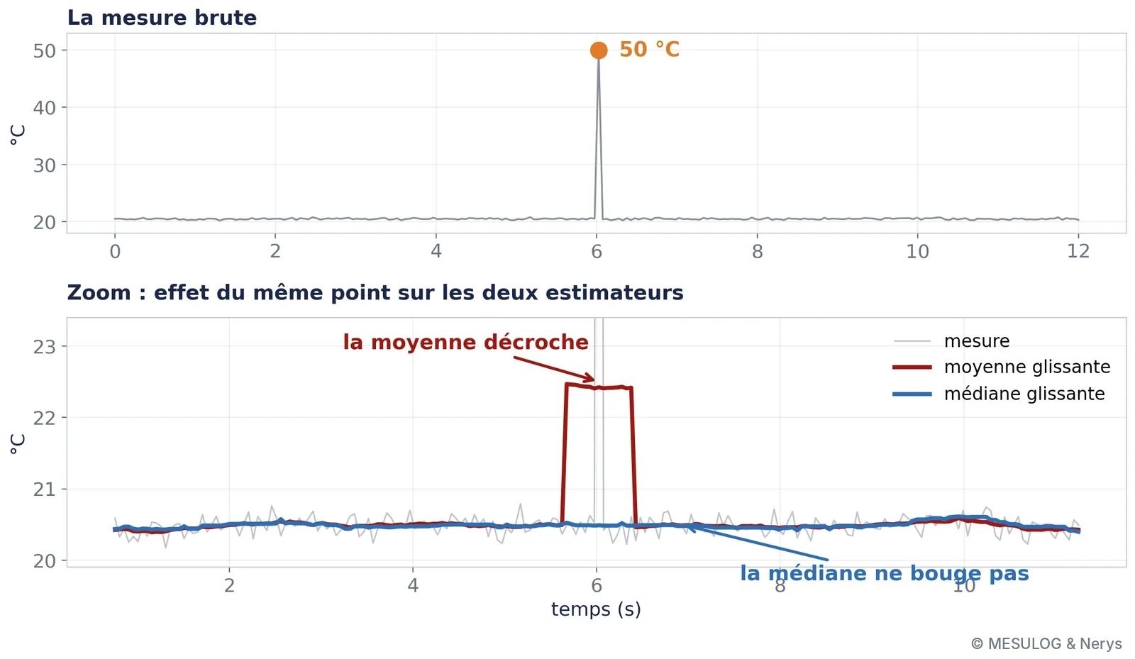
It is not that one is better than the other. They are two different hypotheses about the nature of the noise: the mean assumes symmetrical noise without extreme values, the median assumes that extreme values are rare and meaningless. Choosing one already means deciding something about the phenomenon and about the measurement chain.
The price of smoothing: delay
Then the physical phenomenon really changes: the temperature rises from 20 to 25 °C, then to 30 °C. The filter that protected against noise then becomes a handicap. A 25-point mean or median only follows a step after a dozen samples, half the window, and the mean follows it as a ramp while the median switches abruptly once the majority of the window has changed. The more you smooth, the later you react.
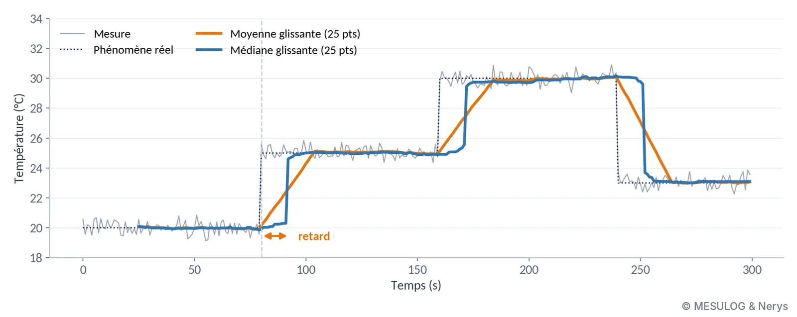
This is the basic trade-off of all processing, and it is not settled by technique. It is settled by answering a business question: how much time do we have to react, and how many false alarms are we prepared to accept? An endurance bench recording an oil temperature over three weeks and a safety loop that must trip within one second do not call for the same filter, even with the same sensor.
NB: the mean itself requires knowing what you are handling. The arithmetic mean of 350° and 10° is 180°, exactly the opposite of reality, whereas both directions are 10° from north. The calculation is right, the tool is right, and the result is wrong, because an angle is a circular quantity. The right method averages the sines and cosines, then recomposes the angle with a two-argument arctangent: you get 0°. The same precaution applies to a phase, a time of day or an encoder's angular position.
2. A spike or a break?
Same signal, one point stands out. Should it be removed or kept? If it is interference, remove it. If it is the first point of a new regime, or the beginning of a break, removing it means masking exactly what you were looking for. On a single sample, the two cases look identical. What happens afterwards is what distinguishes them, and that is what statistics allows you to decide cleanly.
The Gaussian law as a decision rule
If the measurement noise results from many small independent effects, which is the case for thermal noise, quantisation noise and most disturbances in a well-designed chain, its distribution is Gaussian. Two numbers describe it entirely: the mean μ and the standard deviation σ. In the example presented, μ = 20.50 °C and σ = 0.45 °C.
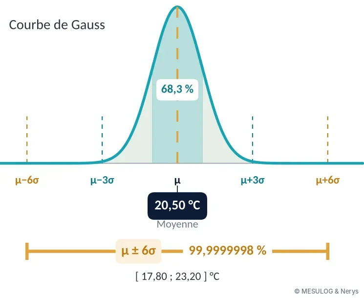
The μ ± 3σ window contains 99.73% of the measurements of a stable regime: one point in 370 falls outside, far too often to trigger a decision. The μ ± 6σ window contains 99.9999998%: about one point in 500 million. At one measurement per second, that is one false alarm every sixteen years. A point outside this window therefore has two plausible explanations: the system has changed, or the measurement is corrupted. In both cases, something must be done.
In the demonstration, the μ ± 6σ window runs from 17.80 to 23.20 °C. A point arrives at 25.5 °C, then a second, then a third: the break is detected, the filter is reset on the new regime instead of smoothing it for 25 samples, and the decision immediately follows the phenomenon.
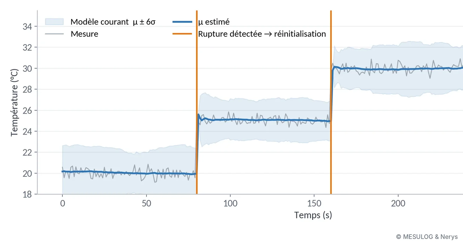
A word of caution: a deviation greater than 6σ does not prove a break. It signals an observation incompatible with the chosen noise model, provided the assumptions of that model hold. If the noise is not Gaussian, if it contains regular impulses or a slow drift, the rule is worthless, and it is the analysis of the measurement chain that must say which noise model to use. We come back to the same sentence: it works because we know what we are looking for.
The same tools to drive the quality of a production line
These tools are used for more than filtering: they measure the quality of a process. On the production benches that Mesulog and Nerys develop with a TestStand test sequencer, each test step is a measurement, with its limits, its verdict and its context (serial number, station, operator). The WATS platform collects these results without re-entry: a reporter connected to TestStand sends each part's report at the end of the test to a centralised database, in the cloud or on the customer's servers. From there, the whole team analyses the same data, from the very first part.
The example presented comes from a real bench: the "Measure VCC" test step, a nominal 5 V supply, with 9,862 measurements collected. The mean is 4.996 V: the process is centred. The standard deviation is about 0.026 V: the μ ± 3σ spread runs from 4.918 to 5.074 V, far from the specification limits set at 4.8 and 5.2 V.
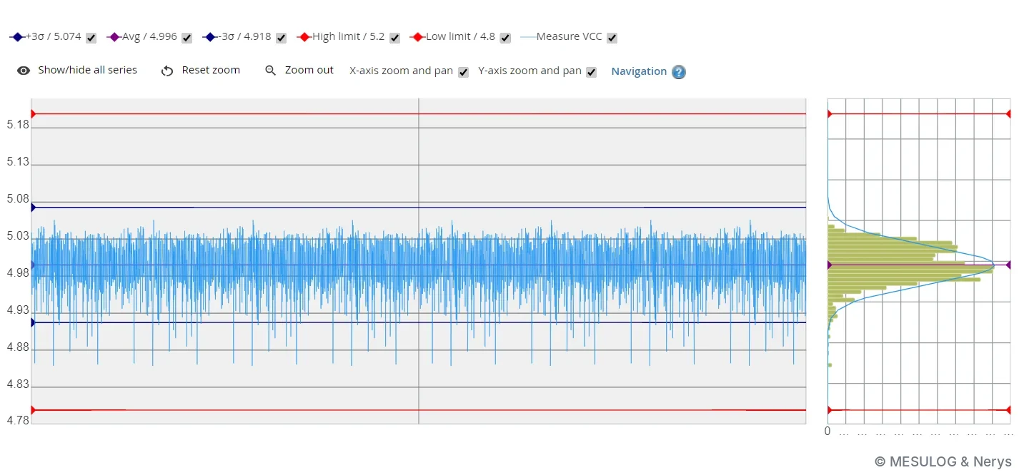
"Far from the limits" is a feeling. Process capability turns it into a figure comparable from one bench to another: Cpk = min[(USL − μ) / 3σ ; (μ − LSL) / 3σ], where USL and LSL are the upper and lower limits. Here, (5.2 − 4.996) / 0.078 ≈ 2.6 on the high side and (4.996 − 4.8) / 0.078 ≈ 2.5 on the low side: the Cpk is about 2.5, where the usual target in production is 1.33. A Cpk below 1 means that part of the production will fall outside the limits even if the process does not drift; a Cpk of 2.5 leaves a comfortable margin, and allows, for example, a discussion about reducing inspection.
Yield indicators complete the picture. FPY (first pass yield) is the rate of compliant products on the first pass; SPY, TPY and LPY track the second, third and last passes. The gap between FPY and LPY measures what retests cost. The Pareto of the ten most frequently failing test steps says where the defects are concentrated, that of the ten lowest Cpks says where to act first, and a CUSUM chart, which accumulates deviations from the target, signals a slow drift before the first failure.
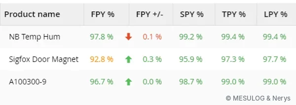
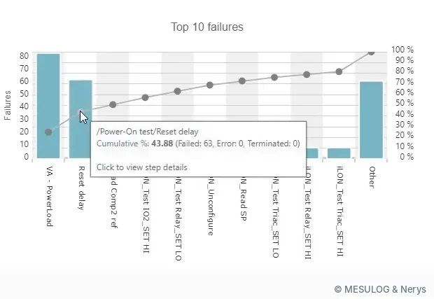
WATS has recently offered two extensions that fall under AI: an integrated assistant that suggests groupings and root causes (by operator, by batch), and an MCP connector that lets an assistant such as Claude or ChatGPT query the test database directly in natural language: "what made the FPY drop last week?", "which stations generate the most retests?". The question is still asked by someone who knows what an FPY is and why it dropped; the tool simply searches faster.
3. The thickness of a slab: linear regression
Third example, a dimensional measurement: the thickness of a marble slab on a conveyor, with a nominal dimension of 20.0 mm. A 2D laser profilometer (a Keyence, in the real set-up) projects a laser line onto the edge of the slab and returns, for each profile, a point cloud of height versus position. A thickness, with its uncertainty, has to be extracted from it.
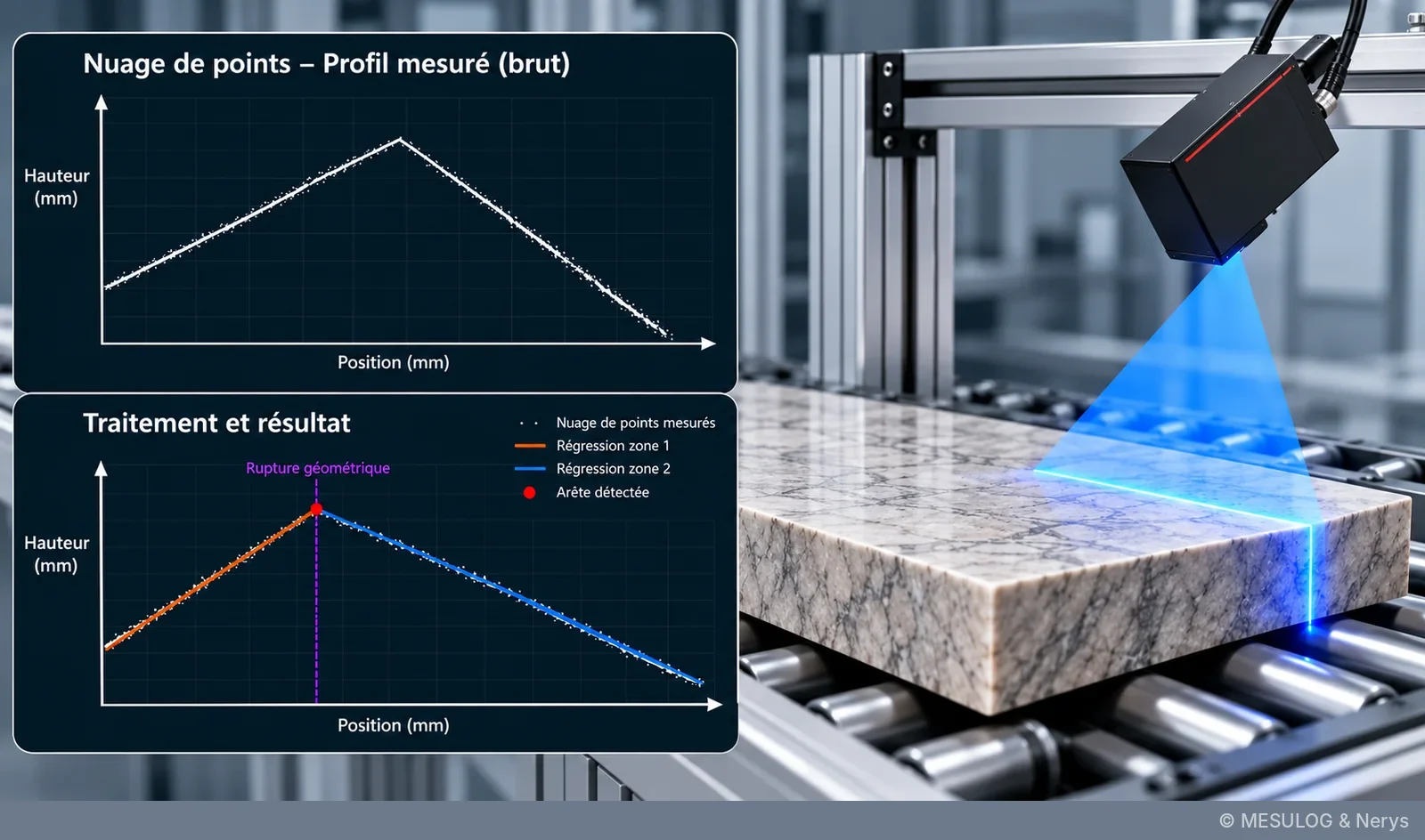
The cloud is imperfect: measurement noise, missing points on shiny or steeply inclined surfaces, a rounded edge that does not give a sharp corner. Taking the highest point and the lowest point does not give a thickness, but the height of the most prominent grain.
The method, in three steps
First step, split the profile into zones: the upper zone, almost horizontal, and the side zone, almost vertical. The boundary is found by looking for the geometric break, the place where the local slope changes abruptly. Second step, model the upper surface by a straight line, fitted by the least-squares method: the line that minimises the sum of the squared vertical deviations between the points and the model. With a few hundred points, the noise of each point averages out, and the line is far more accurate than any isolated point. Third step, calculate the thickness by orthogonal projection of the extreme point of the side face onto this line. The spread of the fit residuals gives, in passing, an estimate of the measurement uncertainty.
Nothing revolutionary: the least-squares method was published by Legendre in 1805. It works because the geometry of the part is known: the upper surface is flat, the edge is roughly perpendicular. On a curved part, the same line would give a wrong result, with larger residuals but a reassuring-looking uncertainty if nobody looks at their shape. Here again, it is knowledge of the measured object that chooses the model.
A linear regression is a neuron
This example also served as a bridge to what followed. A linear regression, y = a·x + b, is a neuron: the coefficient a is the weight, the intercept b is the bias, and the least-squares fit is its training. Everyone in the room had been doing it for years without knowing.
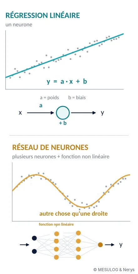
A neural network combines many of these elements, and inserts between them a non-linear function that allows it to represent something other than a straight line. Almost all the methods we now call artificial intelligence are old: regression dates from 1805, control charts from 1924, the perceptron from 1958, backpropagation, which makes multilayer networks trainable, from 1986, convolutional networks from 1989. What has changed is computing power and the volume of available data, not the mathematical nature of the tools.
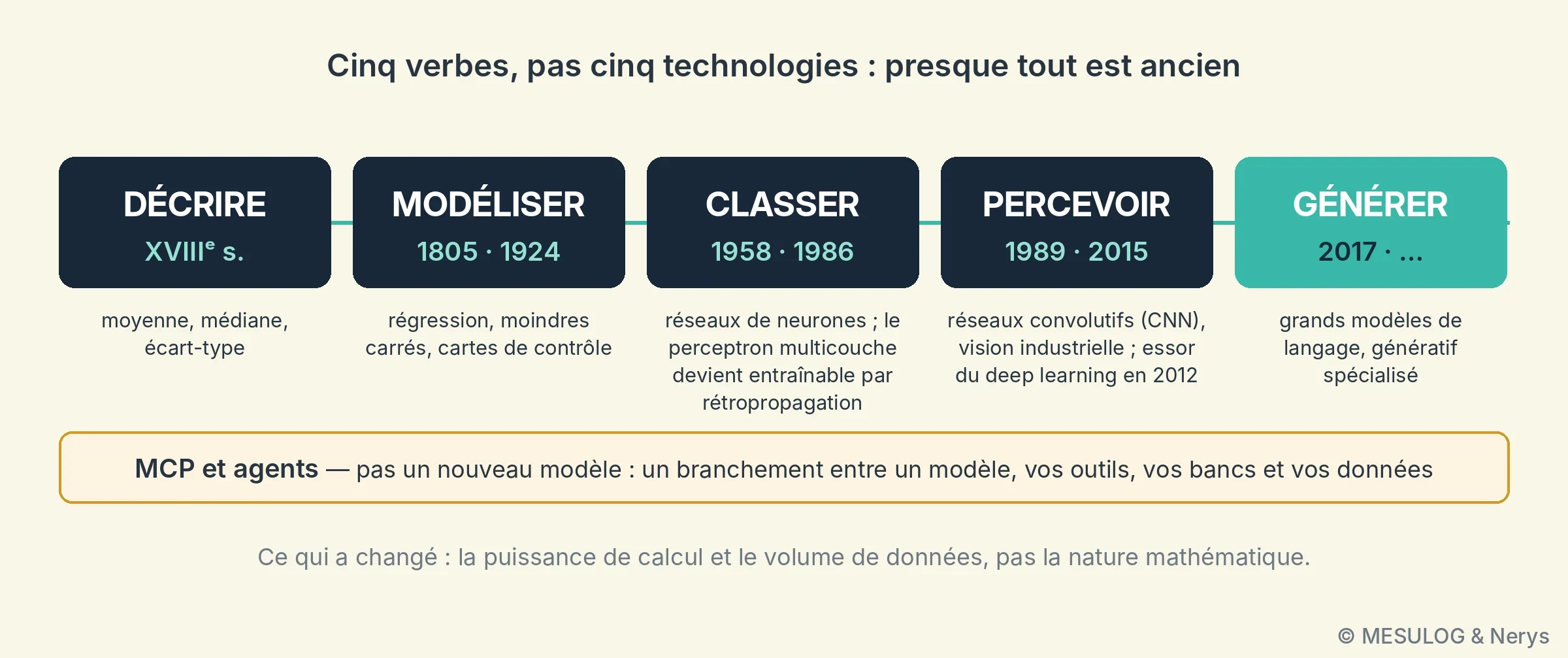
The speakers presented this evolution as five verbs rather than five technologies: describe, model, classify, perceive, generate. Classifying is what decides good or bad at the end of the bench; it has been running at most manufacturers for twenty years, and nobody called it AI. The boundary is fairly arbitrary. As for MCP (Model Context Protocol), it is not a family of models but a connection protocol between a model and your tools, your benches and your data: a plug, not an extra brain.
4. Recognising dice: industrial vision with a neural network
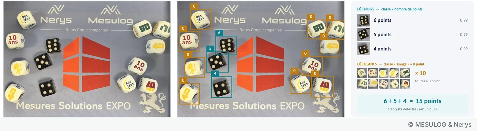
On stand B53, Nerys and Mesulog had set up a game: Human vs AI. The visitor throws two dice into a tray, adds up the visible faces and types the sum on a keyboard; meanwhile, a smart camera identifies the faces, calculates the sum and gives its verdict. The faster of the two wins. The game runs in Vasco, the bench control software published by Nerys: it triggers the camera, retrieves its result, times both players and displays the score. To complicate the task, the tray also contained illustrated white dice, a souvenir of the show's tenth anniversary, which count for zero points.
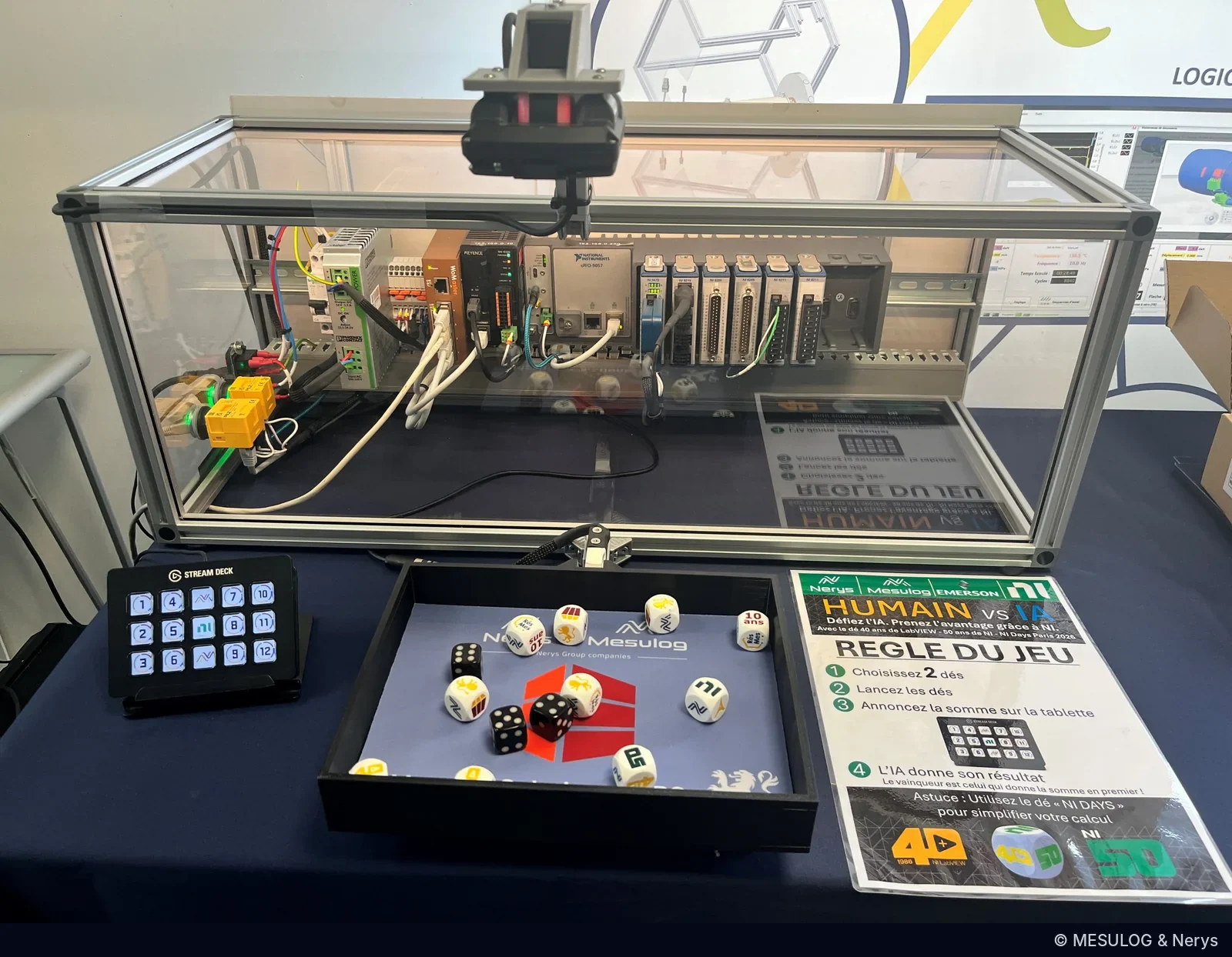
One image, thirteen decisions
Behind the game, an object detection network from the convolutional network (CNN) family, the principle of YOLO-type detectors: from a single image, it locates each object, frames it and classifies it. In the image below, thirteen objects are detected: three black dice, classified "4 points", "5 points" and "6 points" with a confidence of 0.99, and ten white dice classified "image", worth zero. The sum, 15, is not calculated by the network.
Inside the network, the first layers only see contours: on a 64 × 64 pixel thumbnail around a die, eight convolution maps bring out the edges and the dots. The following layers combine these patterns, and the output is not "5" but a probability per class: 96.4% for "5 points", 1.9% for "6 points", 0.9% for "4 points", 0.8% for "image".
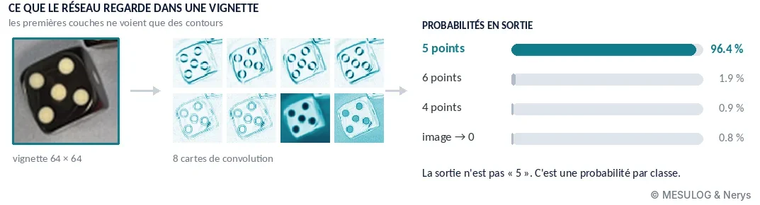
This point has a direct consequence: the AI recognises the objects, it is the software that applies the rules of the game and makes the decision. It checks that there are indeed two countable dice, adds, compares and times; the confidence thresholds, for their part, are set and traced like program parameters. This division applies to any end-of-line visual inspection: the network perceives, the software decides, and the software is verified, versioned and accepted like any other.
What we did not have to do
On the stand, recognition ran in a Keyence IV4 camera, which embeds its own training: no dedicated PC, no code. Configuration is done in four guided steps: optimise the image (triggering, lighting), record a reference image, set up the tools, assign the outputs. The team had defined eight tools: one per die face, one for the total, one for the logo. The complete inspection cycle takes about one second, and the verdict, the count and the match rate come out on I/O and over Ethernet, which Vasco uses directly.
What is surprising is what we did not do: write the network, or program face recognition rules ("count the black spots on a white background…"). You define the objects to recognise, provide annotated images of each face, and the network learns to separate them. When a target is missed in production, the operator frames it on the image, gives it its label and restarts training, in a few seconds.
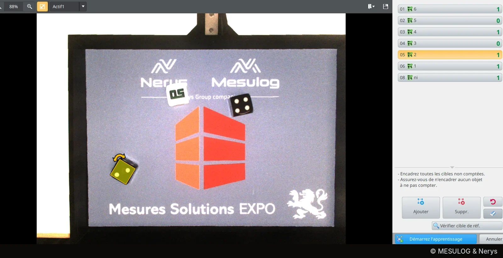
A word of caution, valid for all cameras of this type: retraining is a modification of the inspection program. Who retrained what, when, and on which images, must be traced like a software version. A camera that "learns" without a record is an instrument you can no longer say what it measures.
5. Predicting the zero crossing of a short-circuit current, with Schneider Electric

This is the example Amaury Laurent had to skim over the most, and the one that deserves the most space. It answers a question that sounds absurd put like this: can you act before the signal is there?
A century of testing in Grenoble. To understand the need, a word about the place. Schneider Electric was born in 1836 in Le Creusot under the name Schneider et Cie; the group now has more than 150,000 employees in more than 100 countries, with €40 billion in revenue in 2025. Its Grenoble roots come from Merlin Gerin, founded in 1920 by two Arts et Métiers engineers, Paul-Louis Merlin and Gaston Gerin, around medium- and high-voltage oil-bath circuit breakers. As early as 1921, the company set up a test laboratory, the Volta laboratory, to test its devices at high voltage; it would reach 800 kV in the 1930s. In 1946, Merlin Gerin presented its first circuit breaker able to interrupt a 10,000 A short circuit at 15,000 V, and in the 1960s Grenoble housed one of the largest dielectric test laboratories in Europe. Acquired by Schneider in 1992, the company is now fully integrated into Schneider Electric, which has kept the brand. The Technopole site, in the former Merlin Gerin premises, remains the group's Grenoble heart for switchgear: 1,200 employees, its laboratories and its support functions.
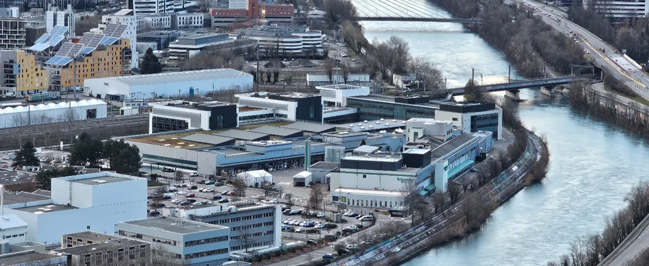
F-Lab and the LEMT. Two main laboratories coexist there. F-Lab is Schneider Electric's test and certification laboratory in France: two platforms in the metropolitan area, Volta in Grenoble and Amplitude in Eybens, 14,000 m² of low- and medium-voltage testing, around a hundred engineers and technicians, COFRAC accreditation to ISO/IEC 17025, and tests carried out under the eye of third-party bodies such as ASEFA or LCIE for product certification. For high-power tests, it has three test generators, two of 600 MVA and one of 2,500 MVA, able to deliver in the order of 300 kA for one second at low voltage; it is this kind of machine that produces the short-circuit currents of this story. Next door, the LEMT, the medium-voltage test laboratory, handles specific tests and developments on switchgear. It is with its teams that Nerys and Mesulog worked.
What these laboratories know how to do, and what they asked for. The site's expertise fits in three words: switchgear, arc physics, test standards. Interrupting a short-circuit current means controlling an electric arc that forms between two opening contacts, with its pre-arc phenomena, and the certification standards precisely describe the conditions under which the interruption must succeed.
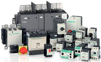
Some of these tests require fast switches to be commanded at a precise instant relative to the current zero crossing, to ensure the transition between high-power sources while limiting the arc energy in the object under test should an arc strike. The commands must be issued several hundred microseconds before the zero, to absorb the latencies of the switching chain, with an accuracy in the order of ten microseconds. The anticipation corrections must be finely and independently adjustable for each action and each phase, including on sequences of closely spaced actions, and some actions must be issued on the microsecond scale when a quantity is exceeded. And all this on a waveform whose frequency and amplitude are both unstable. That is the need as it was put to Nerys and Mesulog.
What the signal imposes. Before any method, the team looked at the laboratory's recordings, acquired at 1 MHz on the short-circuit bench: twelve reference recordings, thirteen usable current channels, peaks of several tens of kiloamperes. No simulation replaces a test campaign, and everything that follows is constrained by what these recordings contain. They impose four constraints.
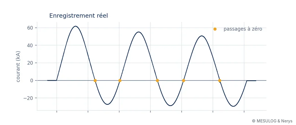
First, an aperiodic component: the circuit is inductive, and the fault current is a sinusoid offset by a decaying exponential whose time constant is around twenty milliseconds. In the test above, the waveform rises to +62 kA on one side and falls to −28 kA on the other; the zeros are therefore not 10 ms apart. Next, the frequency is not 50 Hz: the bench generator slows down under the short-circuit torque, and the team measured from 50.7 to 48.7 Hz depending on the channel. At a 2.6% deviation, a prediction issued 1 ms before the zero assuming 50 Hz is already 26 µs out. In these recordings, the fault lasts only 50 to 65 ms, i.e. three periods: you see the beginning of the slowdown, not its settling. Third constraint, the noise rules out any local method: with a standard deviation of about 48 A before the fault and a slope at the zero going down to 5.9 A/µs, a threshold detection jitters by 16 µs, for a budget of 10. Estimating the frequency on a single half-cycle gives anything between 42 and 60 Hz, because the offset shifts the zeros; over a full period, the asymmetry cancels out and you find 50.1 Hz. You need a model that explicitly separates the offset from the sinusoid. Finally, you must be ready to control 5 ms after the current is established, i.e. a quarter of a period: the estimator is not allowed to converge slowly.
The method, in broad terms. Everything starts from an analytical model of the fault current, which is nothing secret since it is the physics of a short-circuited inductive circuit:
I(t) = a·sin(ωt) + b·cos(ωt) + C + d·e−t/τ
The sine and cosine terms carry the amplitude and phase of the fundamental, C is a residual DC offset, and the exponential term is the aperiodic component, with its time constant τ. The angular frequency ω is not fixed at 50 Hz: it is one of the unknowns.
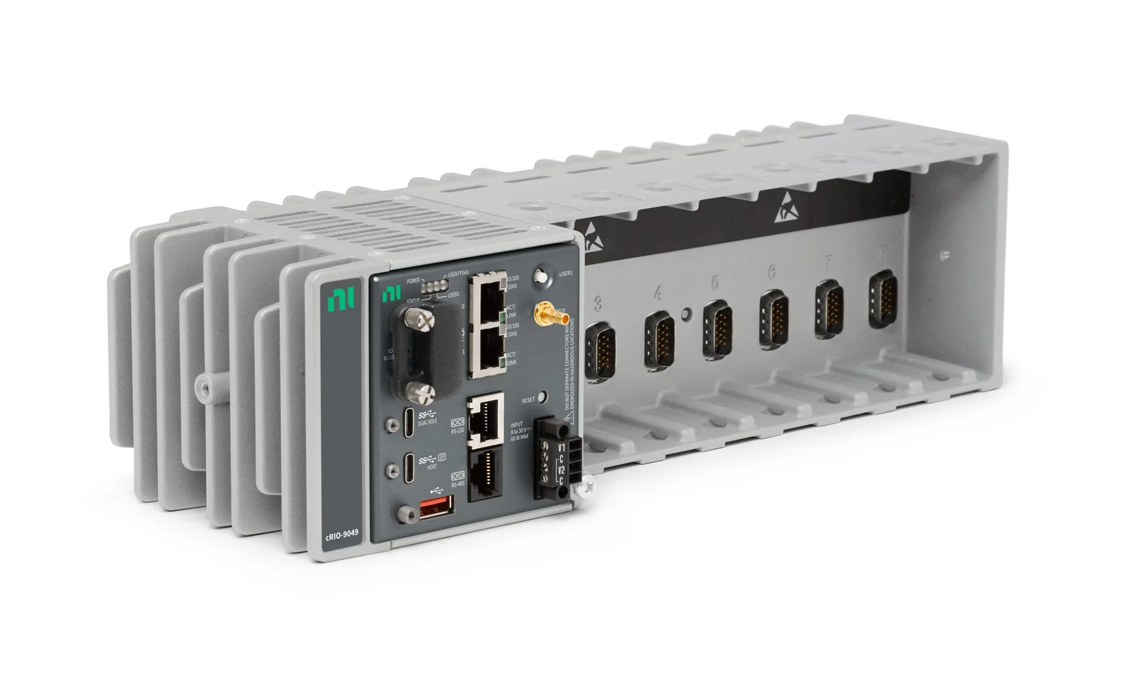
The principle is then to identify these parameters continuously, by least squares, on the samples already acquired. At each new sample, the difference between the measurement and what the model predicts, the innovation, is used to correct the estimate recursively, with progressive forgetting of old samples to follow the evolution of the signal. It is the linear regression of example 3, updated a million times per second. In parallel, a frequency-locked loop corrects the angular frequency: the frequency is tracked, not assumed. Once the parameters are known, the instant of the next zero crossing is derived from the model by a closed-form formula: no search, no iteration. This is what makes the computational cost constant per sample, and therefore compatible with an FPGA processing one sample per microsecond on three simultaneous current channels. In fixed point, the way the recursion is written is not trivial: some classical formulations drift numerically until the estimate diverges, and the team chose one that remains stable. The details of these mechanisms, the weightings and the settings remain between Nerys, Mesulog and Schneider.
The video below replays a real recording from the laboratory. At the top, the measurement and the estimated model, superimposed from the first milliseconds; at the bottom, the distance to the next zero crossing calculated every microsecond. Triggering is requested 100 µs before the predicted zero; the gap between the actual zero and the target instant is displayed at each crossing.
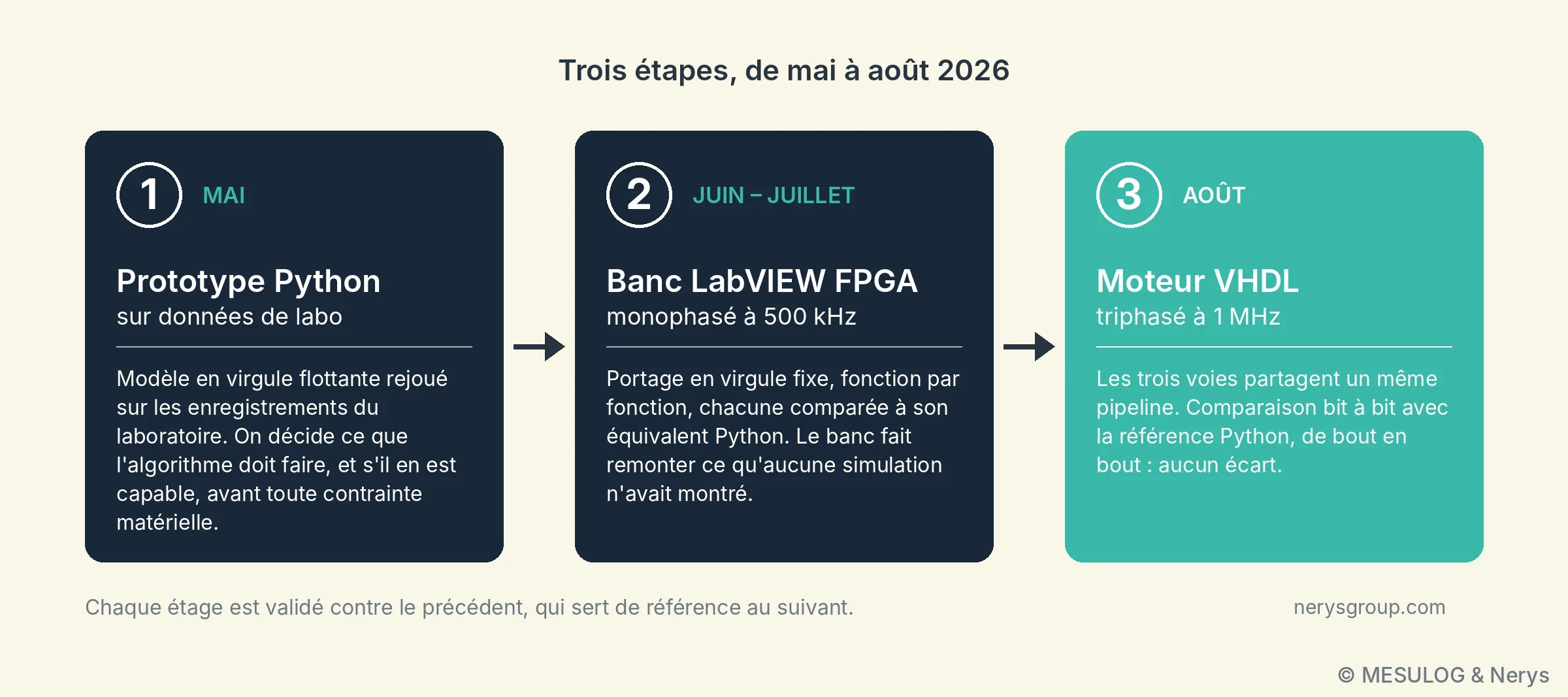
Three stages, from May to August 2026. The integration constraints, FPGA, 1 MHz, fixed point, offer no flexibility for designing an algorithm. The engineers therefore separated the problems. In May, a floating-point Python prototype, replayed on the laboratory's reference recordings: this is where you decide what the algorithm must do and whether it is capable of it, before any hardware constraint. In June and July, a single-phase LabVIEW FPGA bench at 500 kHz: porting to fixed point, function by function, each compared with its Python equivalent on the same vectors. In August, a three-phase VHDL engine at 1 MHz, the three channels sharing a single pipeline, compared bit for bit against the Python reference from end to end: no deviation.
The important word in stage 2 is "bench". Tests on real data brought up what no simulation had shown: detection bounces near the zero, due to converter noise, and fixed-point formats that were too short on some accumulators. This is information that can only come from hardware, and the Schneider team's feedback on real behaviour near the zero redirected several implementation and parameter choices. And the zero bit-for-bit deviation of stage 3 is not a formality: it is what allows us to say that the VHDL does exactly what the prototype does, no more, no less.
How generative AI was used. This is the part that most surprised the room, and the one that must be described precisely so as not to oversell it. The AI did not design the algorithm. It ported an algorithm designed and validated in floating point to fixed point, LabVIEW then VHDL, wrote the test benches and their vectors at the same time as the code, and kept the documentation up to date. What made this possible comes down to three ideas.
The first: the deviation comes back as a number. A harness compares each implementation with the reference, sample by sample, in microseconds and in bits. The feedback is never "it doesn't work", but "at sample 1247, this state diverges by 3 LSB". The harness produces a deviation, not an opinion, and the correction that follows is targeted. The second: what has been understood once is written down. Every pitfall found, an index shift in a recursion, a format that is too short, goes into a file re-read at each session; you do not pay for it twice. The third: the plan comes before the code. The big batches, such as sharing the three channels on a single engine, are specified in a document validated before the first line. You do not correct a direction after 2,000 lines.
The condition for everything else, and what cost the most to build: a bit-exact Python model of the fixed-point arithmetic. Without it, the loop has no sensor, and no iteration is verifiable. The image given by Amaury Laurent is that of a control loop: "the AI produces, the human measures the deviation and feeds it back". What makes the loop stable is that the deviation is a measurement and not an assessment, and that human expertise sets the gain. A loop that does not lock, you stop it, and you start again from a fresh plan rather than piling up fixes.
What remained human. The know-how. The specification and the acceptance criterion. The physical reading of a result, converter noise or real bug. The architecture trade-offs, and the abandonment of leads that did not hold. The bench, the data, and what goes to the customer. In three months, in the order of ten thousand lines of VHDL, three times as much Python model and harness, more than twenty thousand lines of documentation and more than two hundred versioned iterations. The limiting factor was never the speed of writing code, but that of verification; that is where the tool was useful. Each modification was compared with the reference in a few minutes, where a conventional port is verified by simulation campaigns.
Where the accuracy stands. The estimate refines continuously: the later the prediction is issued, the more accurate it is. On the nine channels of the three-phase tests, the median error on the instant of the zero is about 50 µs when the prediction is issued 1 ms before the zero, 15 µs at 0.5 ms, 5 µs at 100 µs and 2 µs at 10 µs. The trade-off is therefore negotiated against the response time of the switching device: the slower it is, the earlier you have to decide, and the larger the error.
With the current settings, the target of less than 10 µs is reached at the closest range on three channels out of nine, and five others lie between 12 and 40 µs. These figures are not final, and the speakers preferred to say so as it is rather than present as settled a result that is not. On the resources side, the three-phase VHDL engine remains bit-for-bit identical to the Python reference, occupies 29% of the Kintex-7 FPGA's DSP blocks and consumes 22 of the 40 clock cycles available for each sample: there is margin left for what comes next.
6. A file of measurements and a generative AI: what works, and what does not
The workshop had started with a show of hands: "who has already asked an AI for something without really knowing what they were looking for?" Hands went up, with laughter. The last example answered that.
The most everyday of the six: a CSV file of measurements as input, a generative AI, and a deliberately vague request, "analyse this for me". The demonstration file contains 200 parts run on an electronic test bench: timestamp, serial number, bench, operator, 3.3 V and 5 V voltages, quiescent current, clock frequency (25 MHz nominal), temperature, RMS noise, test duration, verdict and list of out-of-limit measurements.
The result is impressive. In a few minutes: statistics per column, histograms, breakdown of failures by operator and by bench, correlations, and a formatted Excel workbook with its charts. This is where the Mesulog and Nerys teams save the most time today, without a six-month project: analysing an error log, formatting a report, the first rough pass over a file you are discovering.
But did we get the information that allows a decision? Not necessarily. A starting point, yes; a business analysis goal, no. "This time, it didn't really work, because we didn't know what we were looking for," the speakers admitted. A system asked to find something will always find something: a correlation between an operator and the RMS noise, for example, or a trend that follows the temperature of the day. Just because there are 250 firefighters at a fire does not mean that every event where you see 250 firefighters is a fire. The correlation is real, the explanation is not in the file, and it is the person who knows the bench who knows whether it makes sense.
The difference with example 2 lies there. Asking WATS about last week's FPY drop is asking a precise question of structured data; asking "analyse this for me" is delegating the question itself. The tool is the same, the result is not.
The twist: a stable signal, who signs off?
The workshop ended with a measurement. A signal acquired every day on a bench, flat, clean, repeatable from one day to the next. Question to the room, by show of hands: "this signal is stable, who signs off?" Hands went up.
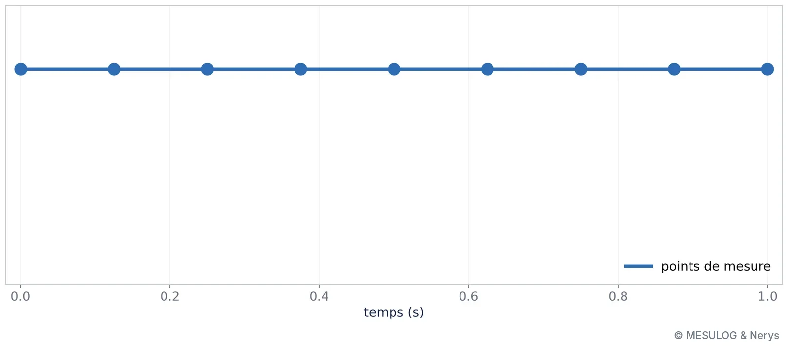
Then the real signal: a clear oscillation, sampled at an unfortunate frequency. The measurement points had not moved. Each sample fell at the same place in the period, so that the whole oscillation disappeared behind a straight line.
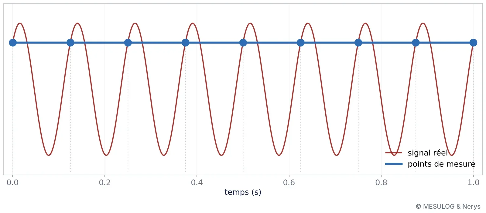
This is not a measurement error: the instrument did exactly what it was asked. It is aliasing. The sampling theorem has said so since Nyquist and Shannon: to represent a signal, you must sample at more than twice its highest frequency. Below that, a fast oscillation folds into a lower frequency, and in the extreme case of synchronous sampling, into a constant. No downstream processing recovers it: not statistics, since the standard deviation is zero, not a convolutional network, not a language model. The remedy is upstream: know the frequency band of the phenomenon, choose the sampling rate accordingly, and place an anti-aliasing filter before the converter. Only knowledge of the physical phenomenon made it possible to see the trap, before the measurement, not after.
Who decides?
The conclusion of the workshop fitted in one diagram: at the centre, the person responsible for the measurement; around them, the consoles — statistics, classification, vision, generative — and the protocols that connect a model to your benches and your data. The engineer is no longer the one who builds the tools: AI has simplified their use so much that anyone can use them. They become the one who manages their power, and they drive it all the better for understanding it. AI is a tool, extraordinarily powerful, but a tool.
There is not statistics on one side and AI on the other. There is a continuum of tools, and an engineer who chooses the right rung of the ladder.
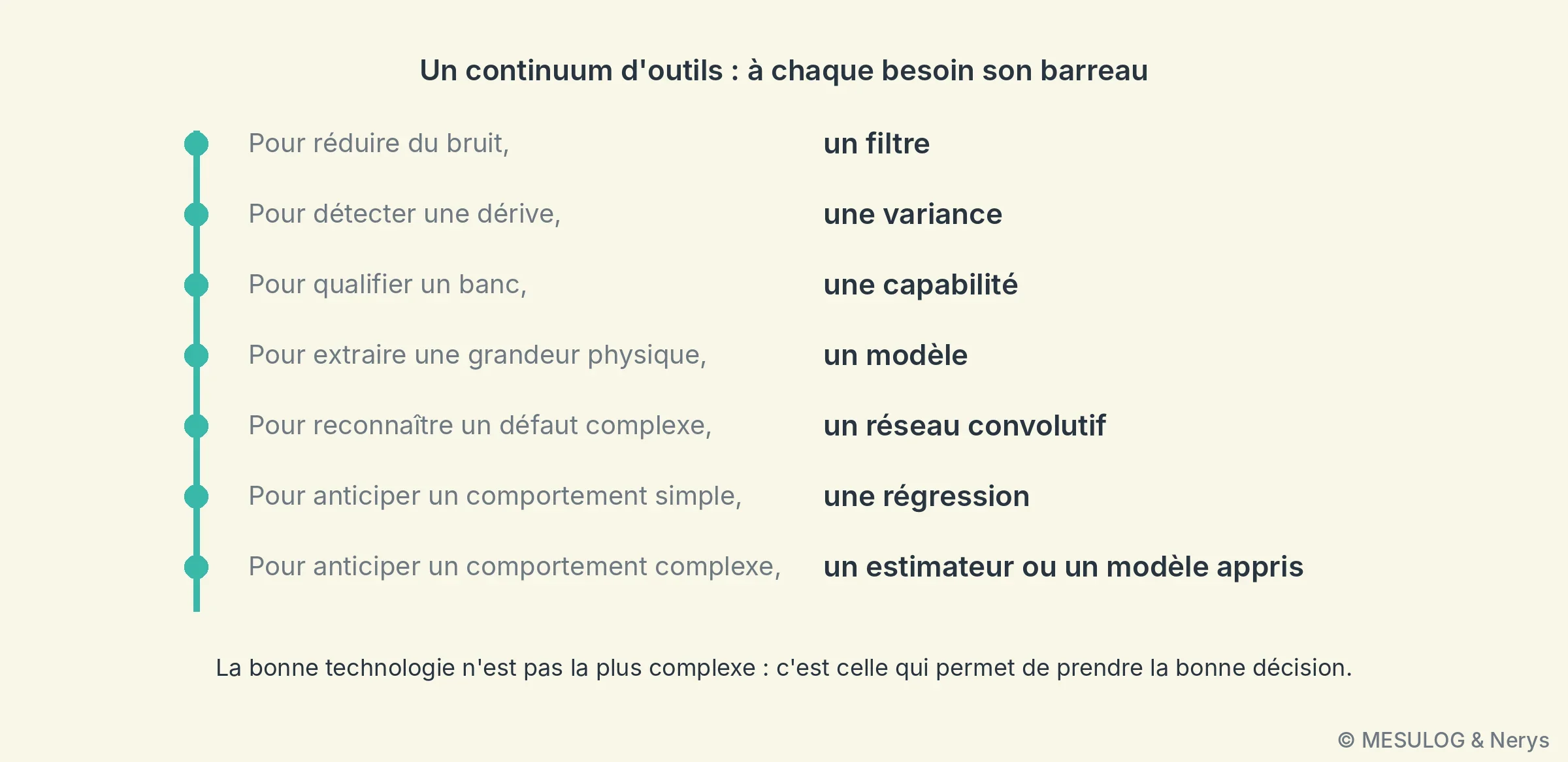
To reduce noise, a filter, mean or median depending on the nature of the noise. To detect a drift, a variance or a CUSUM chart. To qualify a bench, a capability. To extract a physical quantity from a point cloud, a geometric model. To recognise a complex defect, a convolutional network. To anticipate a simple behaviour, a regression; a complex behaviour, an estimator or a learned model. The right technology is not the most complex. It is the one that allows the right decision to be made.
A measurement you don't know what to make of, a signal to anticipate rather than endure? The Nerys and Mesulog teams are happy to talk about it: web@nerysgroup.com.


